This is a read-only mirror of pymolwiki.org
Difference between revisions of "Visualizing a computed structure - a commented example"
Jump to navigation
Jump to search
Qqqqqqqqq9 (talk | contribs) (New page: == The Data == 1. Obtain the data, the following structure was published in http://pubs.acs.org/cgi-bin/abstract.cgi/jacsat/2000/122/i37/abs/ja991878x.html (Supporting Information) 45 ...) |
m (1 revision) |
||
| (6 intermediate revisions by 3 users not shown) | |||
| Line 1: | Line 1: | ||
| − | + | # Obtain the [[Media:File.xyz.tar|File.xyz.tar]] and untar it. It contains the coordinates, which were originally published in [http://pubs.acs.org/journals/jacsat/index.html J. Am. Chem. Soc.] in the Supporting Information of this [http://pubs.acs.org/cgi-bin/abstract.cgi/jacsat/2000/122/i37/abs/ja991878x.html article]. | |
| − | + | # Open the file with PyMOL and save it as a pdb file. | |
| − | + | # Save the following pymolscript [[Media:script.pml.tar|Script.pml.tar]] and untar it to script.pml. Open it with an editor and adjust the Path_To_The_PDB. Open pymol and run the script with "@PATH_Of_The_Script/script.pml". | |
| − | + | # You will get the following image, you can save it with "png filename.png" [[Image:File.png]] | |
| − | + | # Use the script to modify your own pdb-file. | |
| − | + | [[Category:Tutorials|Visualizing a computed structure - a commented example]] | |
| − | |||
| − | |||
| − | |||
| − | |||
| − | |||
| − | |||
| − | |||
| − | |||
| − | |||
| − | |||
| − | |||
| − | |||
| − | |||
| − | |||
| − | |||
| − | |||
| − | |||
| − | |||
| − | |||
| − | |||
| − | |||
| − | |||
| − | |||
| − | |||
| − | |||
| − | |||
| − | |||
| − | |||
| − | |||
| − | |||
| − | |||
| − | |||
| − | |||
| − | |||
| − | |||
| − | |||
| − | |||
| − | |||
| − | |||
| − | |||
| − | |||
| − | |||
| − | |||
| − | |||
| − | |||
| − | |||
| − | |||
| − | |||
| − | |||
| − | |||
| − | |||
| − | |||
| − | |||
| − | |||
| − | |||
| − | |||
| − | |||
| − | |||
| − | |||
Latest revision as of 15:53, 30 October 2015
- Obtain the File.xyz.tar and untar it. It contains the coordinates, which were originally published in J. Am. Chem. Soc. in the Supporting Information of this article.
- Open the file with PyMOL and save it as a pdb file.
- Save the following pymolscript Script.pml.tar and untar it to script.pml. Open it with an editor and adjust the Path_To_The_PDB. Open pymol and run the script with "@PATH_Of_The_Script/script.pml".
- You will get the following image, you can save it with "png filename.png"
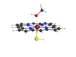
- Use the script to modify your own pdb-file.
